The Rotation Group
Some personal notes and musings about rotations in three dimensions.Portals to page sections:
- Active and passive rotations
- Rotation matrices
- Three-dimensional rotations
- Tensors
- Three-dimensional rotation algebra
- The special unitary group: \(\mathrm{SU}(2,\mathbb{C})\)
- The special unitary algebra: \(\mathfrak{su}(2,\mathbb{C})\)
- \(\mathrm{SU}(2,\mathbb{C})\): double cover of \(\mathrm{SO}(3,\mathbb{R})\)
- Spinors
- Rotors and vectors as matrices
- Quaternions
- Further reading
Active and passive rotations
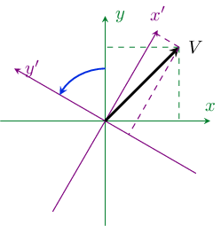
Transformations can be either active or passive.
An active transformation is one that transforms an object.
A passive transformation is one that transforms a coordinate system.
As an example, suppose we have a vector in a plane:
$$
V
=
\begin{bmatrix}
x \\ y
\end{bmatrix}
\,.
$$
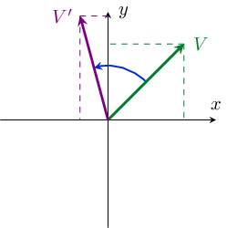
An active rotation is one that rotates the vector itself.
By convention, rotation by a positive angle is counter-clockwise.
Under a rotation by an angle \(\theta\),
a vector transforms as:
$$
V
\mapsto
\begin{bmatrix}
x\cos\theta - y\sin\theta \\ y\cos\theta + x\sin\theta
\end{bmatrix}
$$
This is represented graphically below:
I typically prefer to use active transformations. This is because I think of transformations as acting on specific physical objects. Throughout this (and the other) pages, assume all transformations are active unless I say otherwise.
Rotation matrices
A rotation of a vector in a plane can be represented using a matrix: $$ R(\theta) = \begin{bmatrix} \cos\theta & -\sin\theta \\ \sin\theta & \cos\theta \end{bmatrix} \,. $$ This acts on a vector through matrix multiplication: $$ V = \begin{bmatrix} x \\ y \end{bmatrix} \mapsto R(\theta) V = \begin{bmatrix} x\cos\theta - y\sin\theta \\ y\cos\theta + x\sin\theta \end{bmatrix} \,. $$ Written out in terms of components, the transformation law can also be written: $$ V_a = R_{ab}(\theta) V_b \,, $$ where I'm using the Einsteim summation convention for repeated indices.
Rotations can be compounded through matrix multiplication. A rotation by \(\theta_1\) followed by another rotation by \(\theta_2\) is: $$ R(\theta_2) R(\theta_1) \,. $$ The set of all rotations in the plane forms a group. Formally, a group obeys the following axioms:
- For every pair of group elements \(g_1\) and \(g_2\), \(g_1 \circ g_2\) is also in the group.
- There is an identity element \(1\) for which, given any group element \(g\), \(g\circ 1 = 1\circ g = g\).
- Every group element \(g\) has an inverse \(g^{-1}\) such that \(g\circ g^{-1}=g^{-1}\circ g = 1\).
Three-dimensional rotations
In three dimensions, a vector is represented by a three-component column matrix: $$ V = \begin{bmatrix} x \\ y \\ z \end{bmatrix} \,. $$ Any rotation of this vector is possible to reach by compounding rotations around the \(x\), \(y\) and \(z\) axes. A rotation around any of these axes can respectively be written: $$ \displaylines{ R_x(\theta) = \begin{bmatrix} 1 & 0 & 0 \\ 0 & \cos\theta & -\sin\theta \\ 0 & \sin\theta & \cos\theta \end{bmatrix} \\ R_y(\theta) = \begin{bmatrix} \cos\theta & 0 & \sin\theta \\ 0 & 1 & 0 \\ -\sin\theta & 0 & \cos\theta \end{bmatrix} \\ R_z(\theta) = \begin{bmatrix} \cos\theta & -\sin\theta & 0 \\ \sin\theta & \cos\theta & 0 \\ 0 & 0 & 1 \end{bmatrix} \,. } $$ There are other ways to build up arbitrary 3D rotations. Euler angles are a popular option, and so are quaternions and bivectors.
Rotations around different axes do not commute. A 90 degree rotation around the \(z\)-axis, followed by a 90 degree rotation around the \(x\)-axis, gives: $$ R_x(90^\circ) R_z(90^\circ) = \begin{bmatrix} 1 & 0 & 0 \\ 0 & 0 & -1 \\ 0 & 1 & 0 \\ \end{bmatrix} \begin{bmatrix} 0 & -1 & 0 \\ 1 & 0 & 0 \\ 0 & 0 & 1 \\ \end{bmatrix} = \begin{bmatrix} 0 & -1 & 0 \\ 0 & 0 & -1 \\ 1 & 0 & 0 \end{bmatrix} $$ whereas the same rotations in the opposite order gives: $$ R_z(90^\circ) R_x(90^\circ) = \begin{bmatrix} 0 & -1 & 0 \\ 1 & 0 & 0 \\ 0 & 0 & 1 \\ \end{bmatrix} \begin{bmatrix} 1 & 0 & 0 \\ 0 & 0 & -1 \\ 0 & 1 & 0 \\ \end{bmatrix} = \begin{bmatrix} 0 & 0 & 1 \\ 1 & 0 & 0 \\ 0 & 1 & 0 \end{bmatrix} \,. $$ This can easily be checked with any object lying around. Pick some starting orientation. Revolve it 90 degrees as if it's rolling away from you (the \(x\)-axis rotation), and then 90 degrees counter-clockwise (the \(z\)-axis rotation), and look how it's oriented. Return it to its original orientation, and then perform the two rotations in the opposite order. It'll now be facing a different direction.
The way that transformations fail to commute is one of the most interesting aspects of any transformation group, and receives a lot of focus in group theory.
The three-dimensional rotation matrices are commonly called \(\mathrm{SO}(3,\mathbb{R})\). The S stands for "special," which means the determinant of the matrices is 1. The O stands for "orthogonal," meaning that the matrix transpose gives the inverse. This is apparent in all of the matrices I've written above, but in general any matrix \(M\) in \(\mathrm{SO}(3,\mathbb{R})\) obeys: $$ M M^T = M^T M = \mathbb{I}_{3\times 3} \,. $$
The rotation group is actually part of a special class of groups called Lie groups. In addition to being a group, the rotation group is a differentiable manifold. Rotations are continuously connected to each other by other rotations, and the rotations can be differentiated with respect to \(\theta\).
Tensors
Vectors aren't the only things that transform under rotations. Tensors have their own transformation law.
An example of a tensor is the Cauchy stress tensor, which describes the internal forces felt inside a continuum material in response to strain. The stress tensor is a nine-component object, and can be written as a matrix: $$ \sigma = \begin{bmatrix} \sigma_{xx} & \sigma_{xy} & \sigma_{xz} \\ \sigma_{yx} & \sigma_{yy} & \sigma_{yz} \\ \sigma_{zx} & \sigma_{zy} & \sigma_{zz} \end{bmatrix} \,. $$ For an isotropic fluid, the tensor is diagonal, with all three diagonal components being equal to the hydrostatic pressure. An elastic solid being pulled or compressed in a particular direction will have tension or pressure in one particular direction, so the pressure will be anisotropic. So for instance, the pressure \(\sigma_{xx}\) in the \(x\)-direction might be larger than the other pressures. And some materials experience shear stresses, given by the non-diagonal components.
Components of the stress tensor, like components of a vector, transform under rotation. If you rotate an object that's compressed along the \(x\) axis, the compression will now be in a different direction, and the stress tensor should transform to reflect that. The transformation law for the stress tensor is: $$ \sigma \mapsto R(\theta) \sigma R^T(\eta) \,. $$ Written out explicitly in terms of components, the law is: $$ \sigma_{ab} = R_{ac}(\theta) R_{bd}(\theta) \sigma_{cd} \,. $$ So the vector transformation law is applied to each of the tensor indices separately.
This in principle generalizes further. A rank-\(n\) tensor is an object with \(n\) indices, and for which the vector transformation law applies with respect to each of these indices. The Cauchy stress tensor is a rank-2 tensor in particular. A vector is itself a rank-1 tensor, and a scalar is a rank-0 tensor (since it has no indices and doesn't transform).
Three-dimensional rotation algebra
The Lie algebra of a Lie group characterizes how infinitesimally small group transformations behave. For infinitesimal \(\theta\), rotations around the three main axes can be written: $$ R_a(\theta) = 1 + \lambda_a \theta + \mathcal{O}(\theta^2) \,, $$ where \(\lambda_a\) is called the generator of the rotation. The generators can be written as matrices: $$ \displaylines{ \lambda_x = \begin{bmatrix} 0 & 0 & 0 \\ 0 & 0 & -1 \\ 0 & 1 & 0 \end{bmatrix} \\ \lambda_y = \begin{bmatrix} 0 & 0 & 1 \\ 0 & 0 & 0 \\ -1 & 0 & 0 \end{bmatrix} \\ \lambda_z = \begin{bmatrix} 0 & -1 & 0 \\ 1 & 0 & 0 \\ 0 & 0 & 0 \end{bmatrix} \,. } $$ It is also common (especially in physics) to pull a factor \(-i\) out of the generators, or rather to call $$ J_a = i \lambda_a $$ the generators instead. Both are valid conventions. Using \(J_a\) has the benefit that it can be interpreted as an angular momentum operator in quantum mechanics, which is why physicists prefer to pull out the \(i\).
Regardless of whether the \(\lambda_a\) or \(J_a\) are chosen as the generators, any linear combination of them (with real coefficients) is also an element of the algebra. The generators thus form a basis for the Lie algebra. The Lie algebra for the group \(\mathrm{SO}(3,\mathbb{R})\) is written \(\mathfrak{so}(3,\mathbb{R})\): the same name, but with a lowercase blackletter font.
One of the most important properties of a group is how transformations fail to commute. For a Lie group (such as the rotation group), this can be fully expressed in the Lie algebra in the form of commutation relations. The generators have the following commutators: $$ \displaylines{ [J_x,J_y] = i J_z \\ [J_y,J_z] = i J_x \\ [J_z,J_x] = i J_y \,, } $$ which can be summarized using the Levi-Civita symbol as: $$ [J_a, J_b] = i \epsilon_{abc} J_c \,. $$
The commutation relations tell us how the generators themselves transform under a rotation. Let \(V\) be a vector and \(R_a(\theta)\) be a small rotation around the \(a\) axis (for \(a\in\{x,y,z\})\). Then \(R_a(\theta)V\) is also a vector, and accordingly transforms under another small rotation \(R_b(\phi)\) as: $$ R_a(\theta) V \mapsto R_b(\phi) R_a(\theta) V = \big( R_b(\phi) R_a(\theta) R_b^{T}(\phi) \big) \big( R_b(\phi) V \big) \,, $$ where I've used the fact that \(R^{-1} = R^T\). I've also sorted, into different pairs of parentheses, a transformed vector \(V\) and a transformed \(\theta\) rotation. The rotations themselves transform like rank-2 tensors! In fact, since by hypothesis \(\theta\) is very small: $$ R_b(\phi) R_a(\theta) R_b^{T}(\phi) \approx 1 -i \theta R_b(\phi) J_a R_b^{T}(\phi) \,, $$ so the generators too transform like rank-2 tensors. And using the hypothesis that \(\phi\) is small too: $$ R_b(\phi) J_a R_b^{T}(\phi) \approx -i \phi [J_a, J_b] \,. $$ The upshot is that the commutation relations tell us about how the generators themselves transform under very small rotations. They also tell us that at a deeper level, the reason rotations fail to commute is that the generator of a rotation is transformed by rotations.
Given the Lie algebra \(\mathfrak{so}(3,\mathbb{R})\), it's possible to reconstruct the group through exponentiation. For instance: $$ R_a(\theta) = \exp\{ -i J_a \theta \} \,. $$
The special unitary group: \(\mathrm{SU}(2,\mathbb{C})\)
The special unitary group \(\mathrm{SU}(2,\mathbb{C})\) is the group of \(2\times2\) complex-valued matrices that have a determinant 1 (hence the "special") and for which the Hermitian conjugate is the inverse: $$ M M^\dagger = M^\dagger M = \mathbb{I}_{2\times2} \,. $$ Matrices for which \(M^\dagger = M^{-1}\) are called unitary. This group is intimately tied to the three-dimensional rotation group.
It's possible to write any \(2\times 2\) complex-valued matrix as: $$ M = \begin{bmatrix} a_{11} + i b_{11} & a_{12} + ib_{12} \\ a_{21} + i b_{21} & a_{22} + ib_{22} \end{bmatrix} \,. $$ The Hermitian conjugate is: $$ M^\dagger = \begin{bmatrix} a_{11} - i b_{11} & a_{21} - ib_{21} \\ a_{12} - i b_{12} & a_{22} - ib_{22} \end{bmatrix} \,, $$ while the inverse is: $$ M = \frac{1}{\det(M)} \begin{bmatrix} a_{22} + i b_{22} & -a_{12} - ib_{12} \\ -a_{21} - i b_{21} & a_{11} + ib_{11} \end{bmatrix} \,. $$ Using \(\det(M)=1\) and imposing unitarity means: $$ \displaylines{ a_{11} = a_{22} \equiv a \\ b_{11} = -b_{22} \equiv a \\ -a_{12} = a_{21} \equiv c \\ b_{12} = b_{21} \equiv d \,, } $$ so any matrix in \(\mathrm{SU}(2,\mathbb{C})\) can be written in terms of four real numbers: $$ M = \begin{bmatrix} a + bi & -c + di \\ c + di & a - bi \end{bmatrix} \,. $$ However, these four numbers are not all independent. Imposing once more that \(\det(M) = 1\) tells us: $$ a^2 + b^2 + c^2 + d^2 = 1 \,, $$ meaning that, as a manifold, the group \(\mathrm{SU}(2,\mathbb{C})\) is homeomorphic to the three-dimensional sphere \(S^3\)! The group is therefore simply-connected.
The significance of \(\mathrm{SU}(2,\mathbb{C})\) being simply-connected will become apparent in a bit. Next, we need to look at the Lie algebra to see the connection to the rotation group.
The special unitary algebra: \(\mathfrak{su}(2,\mathbb{C})\)
The Lie algebra \(\mathfrak{su}(2,\mathbb{C})\) consists of \(2\times 2\) traceless Hermitian matrices if the physicists' convention is used for the generators. For a group element \(M\), the corresponding algebra element is \(\mathfrak{g}\), with: $$ M = \exp\{-i\mathfrak{g}\} \,. $$ Unitarity implies: $$ \exp\{i\mathfrak{g}\} = \exp\{i\mathfrak{g}^\dagger\} $$ and having a determinant of 1 means: $$ \exp\{-i\mathrm{Tr}(\mathfrak{g})\} = 1 \,. $$ Unitarity thus implies the algebra elements are Hermitian. Speciality implies the trace is an integer multiple of \(2\pi\). However, we already know that \(\mathrm{SU}(2,\mathbb{C})\) is path-connected (simply-connected, even!), and since \(0\) is an algebra element, it follows that all the algebra elements must be traceless.
The Pauli matrices form a basis for the traceless \(2\times2\) complex matrices: $$ \displaylines{ \sigma_1 = \begin{bmatrix} 0 & 1 \\ 1 & 0 \end{bmatrix} \\ \sigma_2 = \begin{bmatrix} 0 & -i \\ i & 0 \end{bmatrix} \\ \sigma_3 = \begin{bmatrix} 1 & 0 \\ 0 & -1 \end{bmatrix} \,. } $$ Since they form a basis of the algebra, they can be used as generators of the group. More significantly, if we use half the Pauli matrices as the generators, then the commutation relations are: $$ \left[ \frac{\sigma_a}{2}, \frac{\sigma_b}{2} \right] = i\epsilon_{abc} \frac{\sigma_c}{2} \,. $$ This is identical to \(\mathfrak{so}(3,\mathbb{R})\)! Technically, we'd say the algebras \(\mathfrak{so}(3,\mathbb{R})\) and \(\mathfrak{su}(2,\mathbb{C})\) are isomorphic: there is a one-to-one mapping between them that preserves the structure of the algebra (which is fully specified by the commutaiton relations of the generators). As a corollary, the groups \(\mathrm{SO}(3,\mathbb{R})\) and \(\mathrm{SU}(2,\mathbb{C})\) are locally isomorphic, which is just another way of saying that their algebras are isomorphic.
On the other hand, \(\mathrm{SO}(3,\mathbb{R})\) and \(\mathrm{SU}(2,\mathbb{C})\) are not exactly isomorphic, because there isn't a one-to-one mapping between them. In fact, there's a two-to-one mapping from \(\mathrm{SU}(2,\mathbb{C})\) to \(\mathrm{SO}(3,\mathbb{R})\).
\(\mathrm{SU}(2,\mathbb{C})\): double cover of \(\mathrm{SO}(3,\mathbb{R})\)
I'm going to show that \(\mathrm{SU}(2,\mathbb{C})\) maps two-to-one onto \(\mathrm{SO}(3,\mathbb{R})\). The jargon for this is to say it's a double cover.
Let \(S\) be a matrx in \(\mathrm{SU}(2,\mathbb{C})\). There are parameters \(\{\theta_1,\theta_2,\theta_3\}\) for which: $$ S = \exp\left\{ - \frac{i}{2} \theta_a \sigma_a \right\} \,. $$ In terms of these same parameters, we can build a matrix \(R\) in \(\mathrm{SO}(3,\mathbb{R})\) through exponentiation: $$ R = \exp\left\{ -i \theta_a J_a \right\} \,. $$ A map thus exists from \(S\) to \(R\): $$ M(S) = R \,. $$ Basically, just find the \(\theta_a\)'s that give you \(S\), and use them to build an \(R\).
Next, consider a path through \(\mathrm{SU}(2,\mathbb{C})\): $$ S(t) = \exp\{-i\pi\sigma_3t\} = \begin{bmatrix} e^{-i\pi t} & 0 \\ 0 & e^{i\pi t} \end{bmatrix} \,. $$ This is mapped to a path in \(\mathrm{SO}(3,\mathbb{R})\): $$ M(S(t)) = \exp\{-2i\pi J_3t\} = \begin{bmatrix} \cos(2\pi t) & -\sin(2\pi t) & 0 \\ \sin(2\pi t) & \cos(2\pi t) & 0 \\ 0 & 0 & 1 \end{bmatrix} \,. $$ When \(t=1\), the path returns to the identity matrix in \(\mathrm{SO}(3,\mathbb{R})\): \(R(1) = \mathbb{I}_{3\times 3}\). So the path is a loop in the rotation group. On the other hand, it is not a loop in \(\mathrm{SU}(2,\mathbb{C})\): \(S(1) = -\mathbb{I}_{2\times 2}\). In fact, it's not until we go around a second time and \(t=2\) that we return to the same place in \(\mathrm{SU}(2,\mathbb{C})\).
Whereas \(\mathrm{SU}(2,\mathbb{C})\) is simply-connected, we say that \(\mathrm{SO}(3,\mathbb{R})\) is doubly-connected. Every matrix in the 3D rotation group is associated with two matrices in \(\mathrm{SU}(2,\mathbb{C})\), which differ by an overall minus sign. Since \(\mathrm{SU}(2,\mathbb{C})\) is simply-connected, it doesn't have any double covers like \(\mathrm{SO}(3,\mathbb{R})\), and is called the universal cover of \(\mathrm{SO}(3,\mathbb{R})\).
The peculiar double connection of the 3D rotation group can be shown using real-life objects through Dirac's belt trick. Take a belt with a buckle, and clamp the opposite end (without the buckle) into place. The belt represents a path through rotation space: the end clamped in place represents the identity, which is the start of the path. The buckle is allowed to move and rotate freely: its orientation represents the end point of the path. The path itself is represented by the rest of the belt, which must continuously twist to different orientations between that of the buckle and the clamped end. Moving the buckle around doesn't really represent anything, and is just allowed for convenience.
If you twist the buckle around two times (720 degrees), it's possible to undo the twists in the belt without turning the buckle anymore, just by moving it around in space. What you're effectively doing is shrinking the path to a point: if the belt is straight, this means you're not moving through the space of rotations. On the other hand, if you twist the buckle only once from its starting position, you can't undo the twist in the belt without turning the buckle. I recommend playing around with this using a real belt if you never have before.
Spinors
Spinors are mathematical objects that transform under matrices in \(\mathrm{SU}(2,\mathbb{C})\) when rotated. The relevant rotation matrix is: $$ R = \exp\left\{ -\frac{i}{2} \theta_a \sigma_a \right\} \,. $$ Since this is a \(2\times2\) complex matrix, spinors are two-component objects: $$ \psi = \begin{bmatrix} \psi_1 \\ \psi_2 \end{bmatrix} $$ that transform as: $$ \psi \mapsto R \psi \,. $$ In quantum mechanics, the rotation generator can be interpreted as an angular momentum operator. Thus spinors of the forms: $$ \displaylines{ |\uparrow\rangle = \begin{bmatrix} 1 \\ 0 \end{bmatrix} \\ |\downarrow\rangle = \begin{bmatrix} 0 \\ 1 \end{bmatrix} } $$ are respectively considered spin-up and spin-down along the \(z\) axis. In particular, they are eigenstates of \(\frac{1}{2}\sigma_3\) with eigenvalues \(+\frac{1}{2}\) and \(-\frac{1}{2}\), respectively. States that are spin-up or down along different axes can be reached via rotation: a \(90\) degree rotation around the \(y\) moves the \(z\) axis onto the \(x\) axis, and a \(-90\) degree rotation around the \(x\) axis moves the \(z\) axis onto the \(y\) axis. Spin-up and down spinors along the \(x\) axis are thus: $$ \displaylines{ |x:\uparrow\rangle = R_y\left(\frac{\pi}{2}\right) |\uparrow\rangle = \frac{1}{\sqrt{2}} \begin{bmatrix} 1 & -1 \\ 1 & 1 \end{bmatrix} \begin{bmatrix} 1 \\ 0 \end{bmatrix} = \frac{|\uparrow\rangle + |\downarrow\rangle}{\sqrt{2}} \\ |x:\downarrow\rangle = R_y\left(\frac{\pi}{2}\right) |\downarrow\rangle = \frac{1}{\sqrt{2}} \begin{bmatrix} 1 & -1 \\ 1 & 1 \end{bmatrix} \begin{bmatrix} 0 \\ 1 \end{bmatrix} = - \left( \frac{|\uparrow\rangle - |\downarrow\rangle}{\sqrt{2}} \right) \,, } $$ which are indeed eigenvectors of \(\frac{1}{2}\sigma_1\) with eigenvalues \(+\frac{1}{2}\) and \(-\frac{1}{2}\) respectively. Spin-up and down spinors along the \(y\) axis are: $$ \displaylines{ |y:\uparrow\rangle = R_x\left(-\frac{\pi}{2}\right) |\uparrow\rangle = \frac{1}{\sqrt{2}} \begin{bmatrix} 1 & i \\ i & 1 \end{bmatrix} \begin{bmatrix} 1 \\ 0 \end{bmatrix} = \frac{|\uparrow\rangle + i|\downarrow\rangle}{\sqrt{2}} \\ |y:\downarrow\rangle = R_x\left(-\frac{\pi}{2}\right) |\downarrow\rangle = \frac{1}{\sqrt{2}} \begin{bmatrix} 1 & i \\ i & 1 \end{bmatrix} \begin{bmatrix} 0 \\ 1 \end{bmatrix} = i \left( \frac{|\uparrow\rangle - i|\downarrow\rangle}{\sqrt{2}} \right) \,. } $$ and are eigenvectors of \(\frac{1}{2}\sigma_2\) with respective eigenvalues \(+\frac{1}{2}\) and \(-\frac{1}{2}\).
Spinors have the peculiar property that a 360 degree rotation around any axis changes them by a factor \(-1\), whereas vectors are unchanged by such a rotation. In a sense spinors are more fundamental than vectors, and are said to transform under the fundamental representation of \(\mathrm{SU}(2,\mathbb{C})\). Vectors transform under a different, non-fundamental representation. In fact, vectors are sort of like rank-2 tensors with respect to \(\mathrm{SU}(2,\mathbb{C})\)! I'll elaborate in the next section.
Rotors and vectors as matrices
The fundamental representation of \(\mathrm{SU}(2,\mathbb{C})\), which is the universal double cover of the rotation group, are matrices of the form: $$ R = \exp\left\{ -\frac{i}{2} \theta_a \sigma_a \right\} \,, $$ where \(\sigma_a\) are the Pauli matrices. Spinors are transformed through matrix multiplication, which can be represented in terms of components as: $$ \psi_a \mapsto R_{ab} \psi_b \,. $$ What if we had an object \(T_{ab}\) with two indices—a sort of rank-2 tensor? It'd transform as: $$ T_{ab} \mapsto R_{ac} R_{bd} T_{cd} \,, $$ or: $$ T \mapsto R T R^T \,. $$ Since \(R\) is a complex matrix, transposes are a bit inconvenient; Hermitian conjugates are always better when we can have them. But we can employ a neat trick here: it's always the case for matrices in \(\mathrm{SU}(2,\mathbb{C})\) that: $$ \sigma_2 R^T \sigma_2 = R^\dagger \,. $$ It's worth taking the time to prove this to yourself if you haven't. It thus is convenient to define: $$ V = T\sigma_2 \,, $$ which transforms as: $$ V \mapsto R V R^\dagger = R V R^{-1} \,. $$
Now, \(V\) is a \(2\times 2\) complex matrix, and can be written: $$ V = s \mathbb{I}_{2\times2} + \begin{bmatrix} z & x - iy \\ x + iy & z \end{bmatrix} = s + \sigma_a r_a \,, $$ where \(r_a = (x,y,z)\). In princple any of \((s,x,y,z\) can be complex-valued. The \(s\) term remains unchanged under rotations, and is thus a scalar. How do the other components transform?
Take \(s=0\) for now. Under a rotation around the \(z\) axis: $$ V \mapsto \begin{bmatrix} e^{-i\theta/2} & 0 \\ 0 & e^{i\theta/2} \end{bmatrix} \begin{bmatrix} z & x - iy \\ x + iy & z \end{bmatrix} \begin{bmatrix} e^{i\theta/2} & 0 \\ 0 & e^{-i\theta/2} \end{bmatrix} = \begin{bmatrix} z' & x' - iy' \\ x' + iy' & z' \end{bmatrix} \,, $$ and working out the matrix algebra gives: $$ \begin{bmatrix} x' \\ y' \\ z' \end{bmatrix} = \begin{bmatrix} x \cos\theta - y \sin\theta \\ y \cos\theta + x \sin\theta \\ z \end{bmatrix} \,. $$ This is exactly the same transformation law for rotating vectors around the \(z\) axis. You can work out that for the other rotations, too, the components of the matrix \(V\) transform exactly like components of a vector under rotation.
So vectors can be represented using \(2\times2\) complex matrices, and rotations can be represented using the transformation law: $$ V \mapsto RVR^{-1} \,, $$ where \(R\) is a \(2\times2\) complex matrix defined above. That this is even possible is due to \(\mathrm{SU}(2,\mathbb{C})\) being a double cover of \(\mathrm{SO}(3,\mathbb{R})\). This formulation of vector rotation is sometimes used in computer graphics, where the matrix \(R\) is known as a rotor. The formalism these computer folks use is sometimes called geometric algebra (or vanilla geometric algebra), which seems to have become trendy on the internet recently. Geometric algebra seems to be to be a rebranding of Clifford algebra, but with a lot more focus on intuition and visualization.
Quaternions
Quaternions are a four-dimensional number system with three square roots of \(-1\). They're kind of a generalization of complex numbers. Any quaternion can be written in the form: $$ \mathbf{q} = a + b\mathbf{i} + c\mathbf{j} + d\mathbf{k} \,, $$ where \((\mathbf{i},\mathbf{j},\mathbf{k})\) are the square roots of \(-1\): $$ \mathbf{i}^2 = \mathbf{j}^2 = \mathbf{k}^2 = -1 \,. $$ Quaternion multiplication does not commute in general. In fact: $$ \displaylines{ \mathbf{i} \mathbf{j} = \mathbf{k} \qquad \qquad \mathbf{j} \mathbf{i} = - \mathbf{k} \\ \mathbf{j} \mathbf{k} = \mathbf{i} \qquad \qquad \mathbf{k} \mathbf{j} = - \mathbf{i} \\ \mathbf{k} \mathbf{i} = \mathbf{j} \qquad \qquad \mathbf{i} \mathbf{k} = - \mathbf{j} } $$
A few other properties of quaternions. Their conjugate is defined similarly to complex numbers: $$ (a + b\mathbf{i} + c\mathbf{j} + d\mathbf{k})^* = a - b\mathbf{i} - c\mathbf{j} - d\mathbf{k} \,. $$ However, conjugation reverses the order of multiplication---similarly to the Hermitian conjugate for matrices: $$ ( \mathbf{q}_1 \mathbf{q}_2 )^* = \mathbf{q}_2^* \mathbf{q}_1^* \,. $$ The squared magnitude of a quaternion is given by: $$ |\mathbf{q}|^2 = \mathbf{q}^* \mathbf{q} = \mathbf{q} \mathbf{q}^* \,, $$ so: $$ |a + b\mathbf{i} + c\mathbf{j} + d\mathbf{k}|^2 = a^2 + b^2 + c^2 + d^2 \,. $$
Quaternions can be used to perform rotations. They're apparently the standard way to do rotations in computer graphics. The hint at their relevance can be seen in the commutation relations. If we define: $$ \displaylines{ \lambda_1 = \frac{1}{2}\mathbf{i} \\ \lambda_2 = \frac{1}{2}\mathbf{j} \\ \lambda_3 = \frac{1}{2}\mathbf{k} } $$ then the commutation relations are: $$ [\lambda_a,\lambda_b] = \epsilon_{abc}\lambda_c \,. $$ Compare to the commutation relation for the rotation generators. It's almost the same, except for a missing factor \(i\). In fact: $$ [ (-iJ_a), (-iJ_b) ] = \epsilon_{abc} (-i J_c) \,, $$ so the quaternions would be isomorphic to the rotation group generators if we did not pull out the factor \(-i\) earlier.
So, the purely imaginary quaternions—those of the form \(b\mathbf{i}+c\mathbf{j}+d\mathbf{k}\)—are isomorphic to the algebra \(\mathfrak{so}(3,\mathbb{R})\). Exponentiating the quaternions accordingly gives a rotation group. Actually, it gives a group isomorphic to \(\mathrm{SU}(2,\mathbb{C})\) specifically.
The group we get by exponentiating the quaternions is \(U(1,\mathbb{H})\): the group of unitary quaternions. \(\mathbb{H}\) is the standard symbol for the quaternions (the H is for Hamilton). Unitary here just means the quaternion's inverse is its conjugate, so these are also the quaternions of unit magnitude. It's pretty straightforward to see how the set of unit quaternions is homeomorphic to \(S^3\), and how as a group they're isomorphic to \(\mathrm{SU}(2,\mathbb{C})\).
Rotors can all be written as unit quaternions. Moreover, by replacing the Pauli matrices in the matrix representation of vectors by unit quaternions: $$ \displaylines{ \sigma_1 \rightarrow \mathbf{i} \\ \sigma_2 \rightarrow \mathbf{j} \\ \sigma_3 \rightarrow \mathbf{k} } $$ vectors can also be written as purely imaginary quaternions: $$ V = x\mathbf{i} + y\mathbf{j} + c\mathbf{k} \,. $$ Thus the rotor formula: $$ V \mapsto R V R^{-1} $$ can be applied using just quaternion multiplication.
Further reading
Books
- Robert Gilmore: Lie Groups, Lie Algebras, and Some of Their Applications
YouTube videos
- Tibees: Dirac's Belt Trick demonstrated with long hair
- 3Blue1Brown: Quaternions and 3d rotation, explained interactively
- sudgylacmoe: An Overview of the Operations in Geometric Algebra
- Freya Holmér: Why can't you multiply vectors? (video about geometric algebra)
- Kathy Loves Physics & History: Quaternions are Amazing and so is William Rowan Hamilton!